References:
[1] SciPy: Authors: Eric Jones, Travis Oliphant, Pearu Peterson and others: SciPy: Open Source Scientific Tools for Python. Year: 2001 - . URL: http://www.scipy.org
[2] Eric Jones: Introduction to Scientific Python: Enthought SciPy 2007 Conference.
1. Pylab, a review.
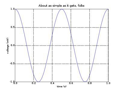
You have already seen many features of Pylab, in particular those related to plotting. This section is a quick review. Matplotlib is a plotting library for Python and its NumPy numerical mathematics extension. It provides the Pylab application programming interface (API) designed to closely resemble that of MATLAB. In a simple example we can show how to make and save a line plot with labels, title and grid:
            from numpy import *
import pylab
t = arange(0.0, 1.0 + 0.01, 0.01) #generate the independent variable values
s = cos(4*pi*t) #define the dependent variable
pylab.plot(t,s)
pylab.xlabel('time(s)')
pylab.ylabel('voltage(mV)')
pylab.title('About as simple as it gets, folks')
pylab.grid(True)
pylab.savefig('simple_plot')
pylab.show()
By now you should not have any problems understanding this code. If we run the program, the output is:
Many functions are shared between scipy and numpy and can be imported from either package. For the time being we will focus on the aspects of scipy that relate to the following functionalities: optimization, statistics and I/O.
2. Scipy Optimization
We often need to solve problems that deal with minimizing the value of an expression under certain constraints. For example, fitting a line to a set of experimentally obtained values requires minimizing the sum of squares of the residuals. The module scipy.optimize provides functions to deal with many such problems and we discuss some applications.
Solving Equations Numerically
It is only possible to exactly determine the roots of a small class of equations. For example, the equation x⁵ - x + 1 = 0 has a real root by the intermediate value theorem, but this equation is not solvable in radicals, and the only way to express the root exactly is to specify that it satisfies that equation. However, we can find approximate values of x that will make the left side of the equation as close as we like to the right side, i.e. we would like to find values of x that sufficiently minimize |x⁵ - x + 1|. Scipy has a function called roots that allows us to do so, but for polynomials only:
            >>> from scipy import roots
>>> coeff = [1, 0, 0, 0, -1, 1]
>>> print(roots(coeff))
[-1.16730398+0.j -0.18123244+1.0839541j
-0.18123244-1.0839541j 0.76488443+0.35247155j
0.76488443-0.35247155j]
We pass the coefficients of the polynomial (starting from that of the highest degree term) as a list or array (in this case, [1, 0, 0, 0, -1, 1] corresponding to our equation 1 * x 5 + 0 * x 4 + 0 * x 3 + 0 * x 2 + (-1) * x 1 + 1 ) and the roots are returned to us as an array. Note that complex roots are returned also. It is important to keep in mind that these values are only approximations of the roots, and sometimes this may make the answers look strange:
            >>> coeff=[1, 2, 1]
>>> print(roots(coeff))
[-1. +3.29272254e-10j -1. -3.29272254e-10j]
You have probably noted that the equation we asked to solve is just x² + 2x + 1 = 0 whose only root is -1.
Many equations we will deal with will not be polynomial equations. There are a number of algorithms to do this and scipy.optimize contains functions for using these algorithms.
One of the more versatile methods to use is fsolve. This function requires an initial guess and it has the advantage that it can solve for the zeros of a general multivariable function
Suppose we want to solve the following system of nonlinear equations:
We will first rewrite this as an expression of the form
and define the function f in Python. Then we will call fsolve to find the zeros:
            from pylab import*
from scipy.optimize import fsolve
def func2(x):
    out=[x[0]*cos(x[1])-4]
    out.append(x[0]*x[1]-x[1]-5)
    return out
x02=fsolve(func2,[1,1])
print(x02)
If we run the program, the output is [6.50409711 0.90841421]. Note that the multivariable function func2 must accept its parameters as a list for this method to work, and the root is also returned as a list. There are other functions in the module that deal with solving equations using different methods. There are also functions that deal with finding the minimal and maximal values of expressions. In fact, the scipy module is just too big to be covered in this tutorial and you will have to learn many of its functions on your own. You will find documentation at: www.scipy.org/Cookbook, but it is a good idea to get used to reading the built-in documentation accessible through the dir and help functions.
Activity 1: Find a solution to the following system of transcendental equations:
The solution is found here. Read through each step and try to understand what is happening.
            from pylab import*
from scipy.optimize import fsolve

def f(x):
    a = exp(x[0]) - log(x[1])
    b = log(x[0]) - exp(-x[1])
    return [a, b]

x = fsolve(f, [1, 1])
print(x) # prints [  1.00000026  15.15427304]
Solving Least Squares Problems
Minimization procedures can be used to solve a least squares problem provided that the appropriate model function is constructed. For example, suppose we want to fit a set of data {(x_i,y_i)} to a known model, y = f(x,p_j) where {p_j} are parameters for the model. A common method for determining which set of parameters gives the best fit to the data is to minimize the sum of squares of the residuals. (see Notes on Error Analysis http:....... for an explanation of the least squares method).
The residual is usually defined for each observed data-point as:
The leastsq algorithm will square and sum the residuals and attempt to minimize the sum by varying the parameters {p_j}. The set of parameters that minimizes the sum of the squares of residuals is returned. We provide an example with a sinusoidal fit.
Suppose it is believed some measured data follow a sinusoidal pattern (for example, such data might be the vertical displacement y of a point on a vibrating string as a function of time). Then our model is:
where the parameters A, T and θ are unknown. The ith residual is:
We will define the function to compute the residuals and guess some starting values for the parameters. The function leastsq will then accept these as parameters to find the best-fit values for A, T and θ.
First we will write some code that will generate a simulation of collected experimental data (how this code works is not relevant to the use of leastsq but make sure you understand it regardless; you should have no problems with this if you use the help function):
            from pylab import *
from scipy.optimize import leastsq
from numpy import random

def residuals(p, y, t):
    err = y - sine_signal(t, p)
    return err

def sine_signal(t, p):
    return p[0] * sin(2 * pi * t / p[1] + p[2])

#number of points in original time series
n = 80

#time dimension: we generate the time values
t = linspace(0, 20, n)
signal_amp = 3.0
phase = -pi/6
period = 6.0

p = signal_amp, period, phase
signal = sine_signal(t, p)

#introduce noise into the signal
noise_amp = 0.2 * signal_amp
noise = noise_amp * random.standard_normal(n)
signal_plus_noise = signal + noise
Now we have a time array and a corresponding array of y – coordinates with some ‘noise’ added that will replicate experimental results (where the data collected is not perfect). We proceed to use leastsq to find the best fit curve and graph the results:
            #initial guess of parameters
p0 = 10 * signal_amp, 1.3 * period, 1.8 * phase

#perform least square fit
plsq = leastsq(residuals, p0, args = (signal_plus_noise, t))

#plot data and fit curve
plot(t, signal, ’bo’)
plot(t, signal_plus_noise, ’ko’)
plot(t, sine_signal(t, plsq[0]), ’ro-’)
legend((‘Signal’, ’Signal+noise’, ’fit’), loc=’best’)
title(‘Fit for a time series’)
show()
The leastsq function accepts as parameters the residuals function and our initial guess of parameters. There is also a third parameter, args=(signal_plus_noise, t). We must use this construction whenever the function we use (in this case residuals) accepts additional parameters. Our function residuals accepts as parameters not just the list p but also the arrays y and t, so we pass these arrays to leastsq in the same order. The returned value of leastsq is a tuple whose first element is the point we are looking for; the other elements of the tuple contain statistical information which we will not look at now. Thus, to access the point (p1, p2, p3), we will write plsq[0]. In the end, we plot the original data, the noisy data and the fit curve.
You may use this code as a template for future problems that involve fitting data. However, since you will be using data collected by experiment, you will generally not need to simulate any experimental data. Do not use this method to generate fake experimental data.
Activity 2: Generate some numbers for the velocity of a ball falling from initial height h = 10 (i.e. use an exact theoretical formula and introduce noise into the numbers). Assume constant gravitational acceleration g = 9.81. Use leastsq to fit the noisy data to a linear model and plot the exact data, the noisy data and the least squares fit.
Here is our solution, although other approaches are possible. Try to make one on your own before reading this.
            from pylab import *
from scipy.optimize import leastsq
from numpy import random

def residuals(p, v, t):
    err = v - velocity(t, p)
    return err

def velocity(t, p):
    return p * t

#number of points in original time series
n = 100

#time dimension: we generate the time values
t = linspace(0, 20, n)

#initial guess for acceleration
p0 = 5
#actual signal
signal = velocity(t, 9.81)

#introduce noise into the signal
noise = 0.1 * signal * random.standard_normal(n)
signal_plus_noise = signal + noise

#perform least square fit
plsq = leastsq(residuals, p0, args = (signal_plus_noise, t))

#plot data and fit curve
plot(t, signal, 'bo')
plot(t, signal_plus_noise, 'ko')
plot(t, velocity(t, plsq[0]), 'ro-')
legend(('Signal', 'Signal+noise', 'fit'), loc='best')
title('Fit for a time series')
show()
3. Statistics
The module scipy.stats provides tools for statistical analysis. Functions are available to generate data samples following certain distributions (with over 80 continuous and 10 discrete distributions available), and the module provides various tools for manipulating data samples. A complete description of the module is available at http://www.scipy.org/SciPyPackages/Stats.
We can use scipy.stats to generate data samples that follow a particular distribution using the rvs function. For example, we can create a normally distributed data sample with mean at 5.0 by typing in the Python shell:
            >>> from scipy import stats
>>> data = stats.norm.rvs(size=10,loc=5.0)
>>> print(data)
[4.35419374  6.24762405  6.24121312  5.53559205  4.01464657  4.22899086 5.97037919  3.87080395  5.34882258  3.2718163 ]
If we omit the second parameter, Python substitutes the default value zero. It is necessary to use the help function to determine exactly what parameters we can pass and what default values are set for these parameters should we omit them. For some other distribution, we would write stats.*.rvs where * is replaced by the name of the distribution in scipy.stats. To just get information about a particular distribution without looking it up elsewhere, we can type print stats.*.extradoc where * will be replaced by the scipy.stats name of the distribution. For example, for a binomial distribution we type:
            >>> from scipy import stats
>>> print(stats.binom.extradoc)
Binomial distribution
   Counts the number of successes in *n* independent
   trials when the probability of success each time is *pr*.
   binom.pmf(k,n,p) = choose(n,k)*p**k*(1-p)**(n-k)
   for k in {0,1,...,n}
Scipy also has functions for performing basic statistical calculations on data samples:
- scipy.mean calculates the sample mean
- scipy.std calculates the sample standard deviation
- scipy.var is the sample variance
The functions mean, std and var take arrays as parameters. We can calculate the mean, standard deviation and variance of all the entries of the array, or just along a particular dimension of an n-dimensional array, in which case we are returned an (n – 1) – dimensional array containing these values. For example,
            >>> import scipy
>>> data = [[1, 2, 3], [4, 5, 6]]  # a 2-dimensional array
>>> a = scipy.mean(data) #calculates the mean of all the values in the array
>>> print(a)
3.5
>>> b = scipy.mean(data, 0) #calculates the means of all the values along one dimension
>>> print(b)
[2.5 3.5 4.5]
>>> c = scipy.mean(data, 1) #calculates the means of all the values along the other dimension
>>> print(c)
[2. 5.]
In general, for an n-dimensional array we can pass a number from 0 to n – 1 to indicate the number of dimensions along which we want to perform the calculation. The same considerations apply to the functions std and var.
The scipy.stats module has many similar functions which are accessible using the dir function.
Activity 3: An exponential distribution is a continuous distribution given by the density function
math
f(x) = \left\{
\begin{array}{ll}
\lambda e^{-\lambda x} & x \geq 0 \\
0 & x < 0
\end{array}
math
Write a program that will generate an exponentially distributed data sample of 100 numbers with parameter λ = 3 (hint: research scipy.stats.expon). Use scipy functions to get the mean of this data sample as well as its standard deviation and variance. Print all these results.
The solution is here: solution_activity_3.py
4. Input and Output
When you collect experimental data, you will generally store it in a table, which will then be stored in an ASCII (plain text) file. The ideal Python construct for storing tabulated data is the array, so in this section we will discuss how to read arrays from ASCII files and how to write arrays to ASCII files. We will use the functions loadtxt and savetxt from the pylab module:
            from pylab import loadtxt
from pylab import savetxt
from numpy import zeros
data = zeros((3,3)) #data is generated as a 3x3 array of zeroes
savetxt("myfile.txt", data) #data is written in an array
data = loadtxt(“myfile.txt")
Try running this program and then examining its results. Note that the function savetxt accepts a path to a .txt file (or simply the filename if the file is located in the same directory as the program) and the array to be written to the file, and does not return anything. The function loadtxt accepts a path to a .txt file and returns the contents of the file as an array.
Example: Create a text file (‘marks.txt’) consisting of your subgroup lab marks:
            weight1        weight2        weight3        weight4
Andy        75                85                80                 90
Sarah       57                70                65                 75
Mitch       80                85                85                 88
We need to read every element of the file except the first row and first column. The numbering of rows and columns starts at 0. We will tell the function loadtxt to read columns 1, 2, 3, 4 by passing to it the construct usecols=(1, 2, 3, 4) and to skip 1 row at the beginning by passing to it the construct skiprows=1. In general, usecols will be followed by a tuple or a list containing the indices of the columns to be read, and skiprows will be followed by an integer indicating how many rows we should skip. We now type in the Python shell:
            >>> data= loadtxt(‘marks.txt’, usecols=(1,2,3,4), skiprows=1)
>>> print(data)
[[ 75. 85. 80. 90.]
 [ 57. 70. 65. 75.]
 [ 80. 85. 85. 88.]]
If we want now to read every other column element we type:
            >>> data = loadtxt(‘marks.txt’, usecols=range(1,5,2), skiprows=1)
>>> print(data)
[[75. 80.]
[57. 65.]
[80. 85.]]
There is also a module called scipy.io that contains functions read_array and write_array. These are deprecated versions of loadtxtand savetxt respectively, however the overall functionality of these functions is not the same. For example, read_array allows us to specify exactly which rows to read, while loadtxt only allows us to skip rows at the beginning of the file. You may choose to use read_array and write_array if you prefer (and documentation is, as usual, available through the help function), but make sure to filter out deprecation warnings to keep the output of your program clean.
Note: Deprecation is applied to program features that are superseded and should be avoided. Although deprecated features remain in the current version of the software, their use may raise warning messages recommending alternate practices, and deprecation may indicate that the feature will be removed in the future. Using deprecated functions results in a deprecation warning being displayed when your code executes. You may avoid this using the following construction at the beginning of your code:
            import warnings
warnings.simplefilter('ignore', DeprecationWarning)
This tells Python to ignore any deprecation warnings so it does not display them when your code executes.
To finish this tutorial, we illustrate a way to use Pylab to import data from ASCII files.
Activity 4. Write the velocity data generated in activity 2 to a .txt file. Then, read this data into an array called read_data and use Pylab to produce a velocity–time graph for the motion.
You may verify your answer with the following example solution: solution_activity_4.py
This concludes our tutorial of the scipy, numpy and pylab modules. There are many more features available that have not been mentioned. You will see some of these in your upcoming coursework. Try the following practice exercises:
scipy.questions.pdf
scipy.solutions.pdf