Contact: compwiki@physics.utoronto.ca

Last updated around: 2021-07-02

1. Introduction

This tutorial will take you through the basics of using Python 3 with the integrated development environment Spyder.

Here is an overview of the software we are documenting on this website:

• Python is a general-purpose programming language that we will use to teach you the use of computers in physics.
• Python has two major versions, Python 2 and Python 3. We use Python 3 but the legacy part of this website documents Python 2.
• Python software is organized in distributions. The distribution we are using is Anaconda Python 3.
• We document how to run Python in an integrated development environment (IDE), which is a software package that lets you test Python commands and edit and run your Python programs. The IDE we are using is Spyder.
• The switch to Anaconda Python 3 and Spyder was done in September 2017. Please read the background page for more information.

We are assuming that Anaconda Python 3 has already been installed on your computer. If this is not the case, go to the "Getting Started" with Anaconda Python 3 page and come back to this tutorial once you've installed the packages.

We use a few formatting conventions to guide you.

• Python commands and output statements are often set in fixed-width fonts, as in print("Hello World!").
• Blocks of code are shaded in grey boxes like this:

            print("Hello World!")
a = 2
b = 3
print("a times b is", a * b)
        

• Code written in these boxes includes coloured highlighting for different parts of the Python language (commands, variables, comments, etc.). If you don't understand the colour highlighting, don't worry about it for now.
• Activities and exercises for you to try are labelled as Activity 1, Activity 2, etc
• Because different IDEs have different prompts at the console, we sometimes omit prompts like In [1]: or >>> for simplicity.

2. Starting Python in the Spyder IDE

During a typical Python session, you will try Python commands interactively, and edit and run Python programs. In these activities, we will start a Python session and run a couple of simple scripts. These scripts are also used in the installation documentation.

Caution about opening .py files: Files that have the extension .py are known as Python scripts. On your computer, these files will appear to be "clickable", i.e. will appear to be files that you can open by clicking them with the mouse. We DO NOT recommend that you open these files by clicking on them. Why? Because quite often the result can be unpredictable. Instead, use the method described below: start Spyder and open Python scripts inside a Spyder session.

Activity 1: Now do the following:

To start Spyder:

• On Windows, a link to Spyder can be found in Start Menu -> Programs -> Anaconda3 (64-bit)
  • You can also search for the Spyder app using the Search window on the Start Menu
  • The simplest way to find it is to search for "Spyder" and click on the icon for the Spyder application.
  • It might take a while (a couple of minutes) for Spyder to start the first time.
  • Please see the install page for more about this.
• On Mac OS X, Spyder can be found in anaconda -> bin -> spyder in your home folder.
  • You can also search for Spyder in Spotlight or use the Anaconda Navigator.
• The result might look something like what is shown below (Mac OS X version from around 2018 shown).

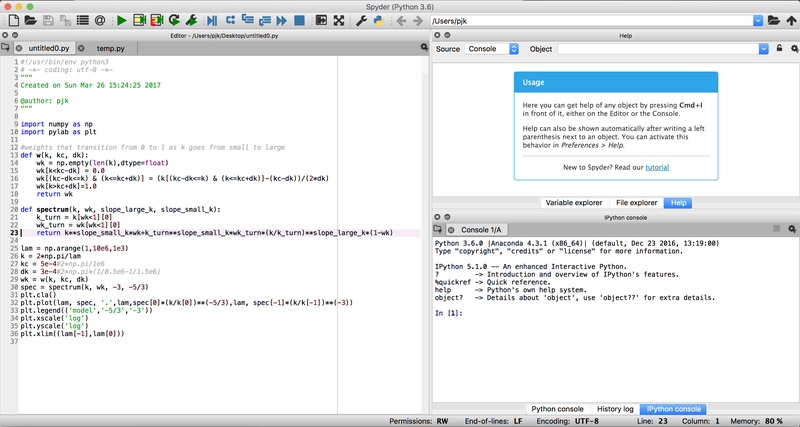
• The initial setup of Spyder reveals three panes (subwindows): 1) a file editor window on the left, 2) a help window on the upper right, and 3) a console window on the lower right. You can adjust the sizes of these pane by dragging the vertical or horizontal bar that separates each pane. You can move them or (accidentally!) delete them using the icons on the top of each pane. You can restore a pane using the View->Panes menu.
• There are a lot of options for configuring Spyder your way, but the first thing to remember is that you can resize these three frames by clicking and dragging.
  • Feel free to experiment with setting the frames in Spyder up the way you like. You might close the "help" window until you need it again.
• Now, Download the histogram demo script, which is taken from the matplotlib examples page.
• Using File -> Open, open this file from inside Spyder and run it by pressing the play button or F5.
• The result might look something like this:

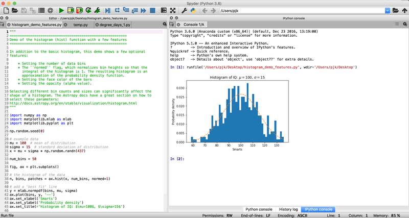
• What's going on? The text edit frame on the left contains the script, and the console frame includes a plot and the new Python prompt (In [2]:).
  • You might have your session set up differently, so that the plotting window appears separate from the console window. If that's the case, don't worry.
  • The histogram might look somewhat different. That's because the version of the script you downloaded is more recent, and uses different data.
• Next, try the same thing with the error bar demo script (also from the matplotlib examples page) and see if you obtain something like

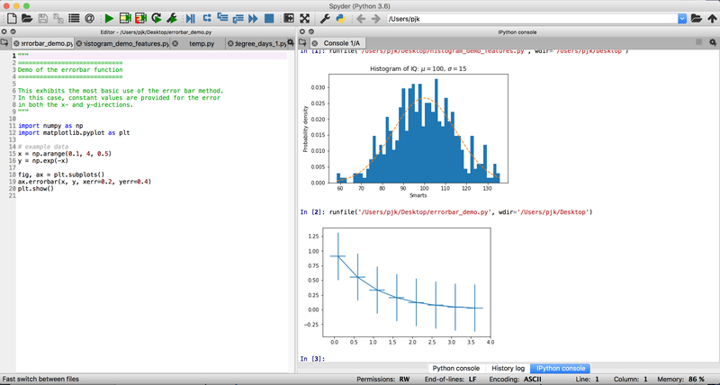
• Now, feel free to open and run any of the scripts in the matplotlib examples gallery. You can click on any thumbnail and learn how to create interesting plots.

When you're done, go on to the next section, where we'll talk about using Python as a calculator and to test code on the fly.

3. Using Python interactively

A "shell" is a computer program that lets you work interactively with a program or an operating system using typed commands. The Console window in Spyder is a shell for Python commands. In the Python shell, you can enter commands for Python to process (or "interpret"). In this section, we will use the Python shell to do some calculations and other work interactively.

Activity 2a: Now do the following:

• If required, using the instructions above, open Spyder.
• Now look at the Console, you will notice that after some technical info, a prompt is displayed.
• It is typically of the form In [1]:, but the 1 could be replaced by some other number. Sometimes, the prompt is of the form >>>.
• Now, at the prompt type

            print("Hello Toronto!")
        

and press return, and you will see

            In [1]: print("Hello Toronto!")
Hello Toronto!
        

(The Console will provide different colours to guide you.)
What just happened? The interpreter was waiting for a command, which you issued by pressing the return key after you typed the text. The interpreter read the command, which asked it to print out Hello Toronto! It didn't see any problems with what you typed, so it responded by following your command.

The Hello Toronto! that appeared in this example is known as a string, which is typically a sequence of characters enclosed by quotation marks (single quotes or double quotes). Strings typically represent information (data, warning messages, etc.) that are meant to be readable. For more advanced information about strings and print statements see Fun with Strings.

Activity 2b: Now what if you made a mistake? Let's see what happens by doing the following:

• Type

            In [2]: print("Hello Toronto!)
        

without the second quote and you will see something like

            In [2]: print("Hello Toronto!)
# some extra stuff appears
SyntaxError: EOL while scanning string literal
        

The interpreter complained (gave a Syntax Error) when it found the end of the command line (EOL) without finding the end of your string with the closing quotation mark. So even though it might have been clear enough to you what was wanted, it wasn't clear to the interpreter and so it didn't print out your command. But notice also --- and this is important --- that your mistake had no other consequences. It didn't destroy Python, or burn out the motherboard of your computer. So don't worry about making mistakes in programming. It just comes with the territory.

Activity 3: Now let's do a simple calculation:

• At the prompt, type

            In [3]: 5.0*2.0
        

and press return. You will see something like

            In [3]: 5.0*2.0
Out [3]: 10.0
        

Activity 3 shows how the Python shell can be used as a calculator; you can scroll up and down in the shell session to look at the calculations you've done. The * is called an operator and there are many of them. We can do standard arithmetic, and a lot more. For example

            In [4]: 5.0/2.0
Out [4]: 2.5
        

The ** operator raises a number to a given power:

            In [5]: 2.0**3.0
Out [5]: 8.0
In [6]: 4.0**0.5
Out [6]: 2.0
        

The latter example took the square root of 4. You can use parentheses to group operations together:

            In [7]: (4.0**0.5)**0.5
Out [7]: 1.4142135623730951
        

You need to be careful with the order of operations you input, which follow Python's "precedence rules". For example,

            In [8]: 2.0 + 3.0 * 5.0
Out [8]: 17
        

calculates 3*5 first and then adds 2. It is a good idea to use parentheses to make things clearer, as the following examples show:

            In [9]: 2.0 + (3.0 * 5.0)
Out [9]: 17.0
In [10]: (2.0 + 3.0) * 5.0
Out [10]: 25.0
        

If it is helpful to you (or anybody reading your code), add parentheses to make your code clear. Even if you are sure the code works as intended without them.

A number like 2.5 with a decimal is known as a floating point number or float, and a number like 2 without a decimal is an integer. In Python 3, the operator / does floating point division, and the operator // does integer division (look online for more discussion of this). There is also the modulo operator %.

Here are various examples of these operators in action

            In [8]: 3//2
Out[8]: 1
In [9]: 3.5//2.5
Out[9]: 1.0
In [10]: 3/2
Out[10]: 1.5
In [11]: 3//2
Out[11]: 1
In [12]: 3.0//2.0
Out[12]: 1.0
In [13]: 3%2
Out[13]: 1
In [14]: 13%3
Out[14]: 1
In [15]: 13%4
Out[15]: 1
In [16]: 13%8
Out[16]: 5
        

Activity 4: To test this behaviour do the following:

• Predict the result of the following print statement using quotient and modulo statements.

            In [17]: print(9//4, 9.0//4, 9.//4, 9/4, 9.0/4.0, 9%4, 9.%4, 1/2, 1//2, (3.0**2)//(2.0**2))
        

and check your prediction by typing the command.

• Notice the following:
  • The regular quotient always results in a float, and the integer quotient results in an integer, unless one or both of the numerator or denominator are floats.
  • The trailing zero after the decimal point can be omitted, so that 5. is equivalent to 5.0.

Activity 5: Here's another exercise:

• Predict the result of the following calculation

            (2.0/4.0)**(1//2)-(13.0/14.0)**(5//2-7//3)
        

and check your prediction by typing the command.

Now, let's write a little code to calculate a formula in physics. From first year mechanics, we know that an object projected upward with speed v will reach a height

in the absence of air resistance. Suppose you throw a ball with a vertical component of velocity of 12.5 m/s. The following calculates the height reached:

            In [18]: 12.5**2/(2*9.8)
Out [18]: 7.971938775510203
        

So the ball rises about 8 meters.

Introducing Variables and Assignment Statements

Another person looking at the statement In [18] in the previous example would have no idea what the calculation means. To produce clear work that anyone can understand, we need to use variables.

Activity 6: Let's redo the previous example using variables.

• Type the following commands one at a time, pressing return after each command. For simplicity, we will drop the prompts In [19]:, Out [19]: etc.

            v=12.5
g=9.8
h=v**2/(2*g)
print(h)
        

In these expressions, the interpreter assigns a value to v and g, and assigns h a value based on the values of v and g. The formula for h and the dependence on the variables are clearer now. The last line printed the value of h:

            print(h)
7.9719387755102034
        

The variable h in this example refers to a specific number and not a symbolic formula. As a result, if you change v or g, the value of h won't change, even if we originally set h by a formula involving v and g. To see what we mean, try typing the following:

            v = 15
print(h)
7.9719387755102034
        

The point here is that h stays the same, even though v has been changed. To update h to reflect the new v, we need to repeat the formula:

            h = v**2/(2*g)
print("The height of the ball h =", h)
The height of the ball h = 11.479591836734693
        

So for a starting velocity of 15 m/s, the ball rises about 11.5 m.

The statement h=v**2/(2*g) is an assignment statement, and we will stop for a bit and think about what it means. In this statement, the equal sign = is telling the Python interpreter to take the numerical value of the calculation v**2/(2*g) and assign it to the variable h. Until we write another assignment statement with h on the left-hand side, the value of h does not change.

Assignment statements can be chained together to update a variable without creating a new variable. For example, on my birthday, my age is increased by one year. The following commands would be good for marking my birthday.

            age = 42
print( "Your current age is", age)
Your current age is 42
age = age + 1
print( "Happy Birthday! Your new age is", age)
Happy Birthday! Your new age is 43
        

A short form for the construction age = age + 1 is age +=1. Similarly,

• a = a - 1 is equivalent to a -= 1,
• a = a*2 is equivalent to a *=2
• a = a/2 is equivalent to a /= 2

Activity 7: Now do the following:

• The activity of radiatioactive decay for a given sample (Knight, Second Edition, Chapter 43) is given by

where \(R_0\) is the activity at \(t=t_0\) and \(t_h\) is the half life.

• You can use this formula to show that

[Don't worry if you don't understand these expressions completely. Just take them as given.]

• The half life for Cesium-137 is 30 years (Knight, Second Edition, Example 43.3). Given an initial activity of 5.0µCi (microcurie), write some code that will print the activity in microcuries every 10 years for four or five decades.
• One way to approach this problem is to first define a variable fac that represents the constant \(\left(\frac{1}{2}\right)^{(\Delta t/t_h)}\) that appeared in the half-life equation. Notice that this constant is independent of time t but depends on the elapsed time ∆t. Then define a variable r that represents the initial activity. Then the assignment statement r = r * fac or r *= fac updates the activity to its value after time ∆t. Repeating this assignment statement will give you the activity every ∆t.

A sample session in which we solve this problem can be found in the following (prompts omitted):

            r = 5.0
t12 = 30.0
deltat = 10.0
fac = 0.5**(deltat/t12)
print('Initial activity', r)
#Initial activity 5.0
r = r * fac
print('Activity is now ', r)
#Activity is now  3.968502629920499
r = r * fac
print('Activity is now ', r)
#Activity is now  3.149802624737183
r = r * fac
print('Activity is now ', r)
#Activity is now  2.5000000000000004
r = r * fac
print('Activity is now ', r)
#Activity is now  1.9842513149602499
        

4. Using Python Scripts

We have been using Python interactively for these first quick answers and examples. Interactive shell sessions are nice for trying a couple of commands in a row. But if you need to chain together a sequence of several commands, as in the last exercise, it is much more efficient to save them to a file and use Spyder to run the file. A set of Python commands in a file is called a script. Like a movie script for an actor, the Python script tells the Python interpreter what to do and in what order to do it.

First, we'll introduce comments, which are lines of text that are ignored by the Python interpreter but that are included to help explain your code to others and to remind yourself what your code is intended to do. Good code writing requires good comments. Comments in Python start with a # sign. Any text following the # sign is ignored by the interpreter. For example, if you cut and paste the following command into the Python shell, the text after the this print statement will not be printed.

            print ("This is a print statement.")  # This comment will not be printed.
        

(Notice that the color highlighting in the code block makes comments appear grayed out. This is the type convention followed by the wiki software we are using; some people find the comments hard to read as a result.)

Activity 8: Now we will save some commands to a file and run the file as a Python script.

• First, open a new file from within Spyder, by going to the file menu and pointing to File → New.
• We will redo our previous projectile example as a script. In the script window, enter the following commands by either cut-and-pasting or typing:

            # Initial vertical velocity... A comment to start things off!
v = 15.0
# Gravity
g = 9.8
# height formula
h = v**2/(2*g)
# print result
print("If v = ", v, " and g = ", g, " then h = ", h,".")
        

• [Again, the colour highlighting in the code box is intended to guide you. You can cut and paste this code into a script without worrying about the colours.]
• Now, save the script to a location of your choice. Call it vgh.py, or some other name you prefer.
• (We repeat: It is important that you save your code with the extension .py.)
• Then, run the script. There are two ways to do this:
  1. You can go to the Run menu and select Run → Run Module or
  2. You can type F5.
• This will run the module and should produce the following output in the interpreter:

            If v = 15.0 and g = 9.8 then h = 11.4795918367.
        

Your session might look something like this (or more recent),

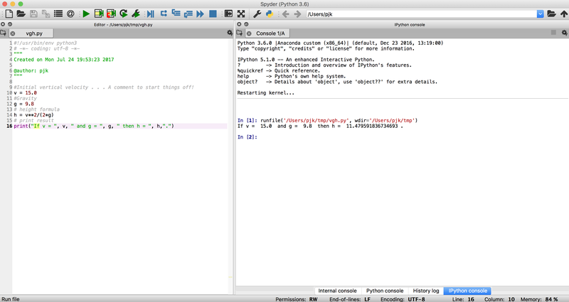
In the text editor frame, we've entered the commands, and you can see that Spyder has coloured the text using its syntax highlighting. (It does this in both the shell and file windows.)

The script consists of the set of commands you have already run interactively. We have added comments that start with # to help document the code.

When you selected Run or typed F5, several things happened. Run or F5 is a command that asks Spyder to translate (compile) the code into a form the computer can understand, load the translated code into the computer memory, and run the commands in the script one at a time in the order they are written. You as a user should understand the following about Run or F5:
1. Spyder will typically run each separate line in your script as a command. That is, the script executes all the command sequentially, in the order that they are written.
2. It skips every comment line in the script.
3. Once it is finished, it returns a prompt. This means that is now waiting for further instructions. You can now go ahead and type additional commands interactively.

Activity 9: Create and run another script for practice.

• Redo Activity 7, using a script instead of interactive commands. At each time increment ∆t, print the current time as well as the activity.
• A sample script can be found here - you can download and run this script.

Mistakes, Bugs, Errors, Warnings: It is sad but true that most of your time in programming will be spent debugging --- finding and fixing coding errors. Strategies for debugging are covered here in the Python Reference, but this is a good point to say something about Spyder's debugging hints. You will find that when a code contains errors that are obvious, Spyder will try to inform you that it sees the problem and will try to identify where the problem might be. This will become more apparent as you start working with the text editor. If you pay attention, you will also see that the editor will provide hints for the next things you might type, etc..

Activity 10: Consider the following set of inputs:

            a = 2
b = 3.0
ab = a b
print(my_new_variable)  # my_new_variable has never been defined
        

• Do you see where the syntax error is? Do you see another problem? What did Spyder do to point out the problems in each case?
• Now enter the lines one at a time in the Python shell. What do you find?
• Now, copy and paste the commands above into a script, and notice how Spyder gives you some clues as to the potential problems.

5. Summary and Conclusions

This section

• Started out with some background on our setup and this tutorial.
• Then introduced how to start Anaconda Python using Spyder and run programs from it.
• Showed you how to work interactively with Python and how to create and run scripts. Hopefully you are now getting comfortable with Spyder and the Console (Python shell). Feel free to explore the Spyder IDE in more depth or look for other environments that work better for you.
• Introduced operators +, -, /, //, *, etc... within the shell. The operator = is a powerful tool, it can be used in Python to both assign and modify variables, which in turn can be used to clarify formulas.
• Introduced comments, which are a vital part of programming in any language. It is considered proper form to put a comment beside any confusing piece of code you may write. This helps both you and anyone else reading the code if ever a part of code needs to be reused and its purpose is forgotten.
• The final section of this part of the tutorial covered making and saving .py programs outside the shell, and running them from with Spyder. If you are not comfortable doing this, go back and reread that part of the tutorial. Making and using .py files will be necessary to complete 90% of the remaining portion of this tutorial.

Here are some questions about the all the material covered in this section (current links are for Python 2 documentation):
Part_1_Questions.pdf

Part 1 Solutions.pdf

This concludes Part 1. Now proceed to Tutorial Part 2, where you will learn more about Python commands and packages (modules).