Learning Physics with PyLab

Preliminary warning: this page contains some deprecated instructions, and overall, is about the use of a module that is typically not recommended. Follow at your own risk.

This tutorial will provide you with the additional tools you need to use Python in our second year courses. We will explore PyLab, which uses NumPy and the plotting packages of Matplotlib. Because these two modules are 90% of what an undergraduate Physics student needs, PyLab can be very convenient and many examples in your courses use it, although its use is typically not recommended. We will still walk you through the basics.

Outline:

Getting your work done with PyLab: plotting, formatted output, reading in data from a file.
Working with NumPy.

1. Getting your work done with PyLab

In your second year courses, you will be using PyLab to get work done in a variety of ways. We tested PyLab in the First Steps, Part 2 tutorial.

Plotting in PyLab

Let's start with a look at the basics of plotting. Look at the following code:

python code

            # import numpy functions and types
from pylab import *
plot([1,2,3,4],[1,4,9,16])
show()

This code will simply plot the elements of the list [1, 2, 3, 4] against the elements of the other list [1, 4, 9, 16]. The final command in all PyLab plotting should always be show(), which activates the plotting window. Conversely, avoid calling show() before the very end of the script.

Activity 1: Copy and save the excerpt above to a new script file, and run it in IDLE using F5. The result should be a window like this

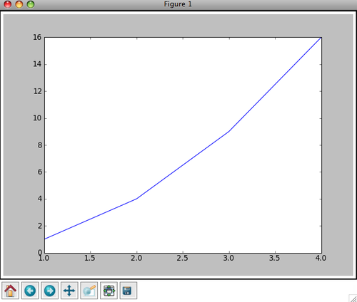
Notice the row of icons at the bottom of the window. These icons allow you to explore your plots by panning the plots and changing its settings. For more information on these buttons see the interactive navigation documentation at http://matplotlib.sourceforge.net/users/navigation_toolbar.html.

To learn more about the very powerful plot command, in the Python shell type

from pylab import * help(plot)

The following activity will help you explore several useful capabilities of Matplotlib.

Activity 2: Do the following:

Copy and paste the following script into a new IDLE script window and run it. Resize the plotting windows to view them properly, if necessary.
Close the plotting windows, then quickly read over the code, trying to get an overall understanding of the different commands.
For guidance on the commands, type from pylab import * in the Python shell and use help() on the commands. This is a quick way to learn about the capabilities of PyLab.

python code

            # import numpy functions and types
from pylab import *
x = arange(1,10,0.5)
xsquare = x**2
xcube = x**3
xsquareroot = x**0.5
# open figure 1
figure(1)
# basic plot
plot(x,xsquare)
# add a label to the x axis
xlabel('abscissa')
# add a label to the y axis
ylabel('ordinate')
# add a title
title('A practice plot.')
# save the figure to the current diretory as a png file
savefig('plot_1.png')
# open a second figure
figure(2)
# do two plots:
# one with red circles with no line joining them
# and another with green plus signs joined by a dashed curve
plot(x, xsquare, 'ro', x, xcube,'g+--')
# x and y labels, title
xlabel('abscissa')
ylabel('ordinate')
title('More practice.')
# add a legend
legend(('squared', 'cubed'))
# save the figure
savefig('plot_2.png')
figure(3)
# use the subplot function to generate multiple panels within the same plotting window
subplot(3,1,1)
# plot black stars with dotted lines
plot(x, xsquareroot,'k*:')
title('square roots')
subplot(3,1,2)
# plot red right-pointing triangles with dashed lines
plot(x, xsquare,'r>-')
title('squares')
subplot(3,1,3)
# plot magenta hexagons with a solid line
plot(x, xcube,'mh-')
title('cubes')
savefig('plot_3.png')
# show() should be the last line
show()

The result will produce a session that looks like this, after rearranging and resizing the windows:

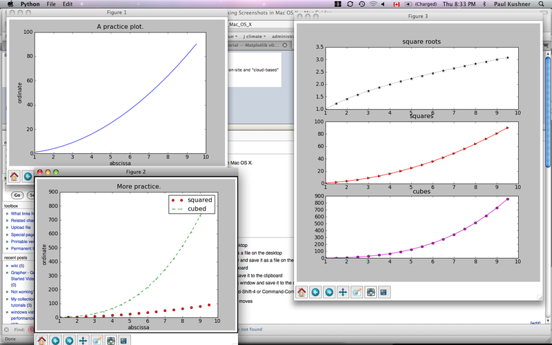
This code demonstrates a lot. It shows examples of:

Plotting with numpy arrays, defined based on the arange() command.
How to open multiple plotting windows with figure()
How to add plotting symbols and change the lines joining the points with strings like 'ro' (red circles) and 'g+--' (green plus signs with dashes). For more information on plotting, type help(plot) and see the Matplotlib tutorials.
How to save your plot to a graphics file with savefig(). To save to a pdf, replace the .png suffix with .pdf.
How to label and title your figures with xlabel, ylabel, title.
How to use the subplot command to create multiple window figures. The basic syntax for subplot is subplot(rows, cols, num), where rows is the number of rows in the plot, cols is the number of columns in the plot, and num is the plot number. See help(subplot). The example shows three plots in a single column.
That you should use show() on the last line of code.

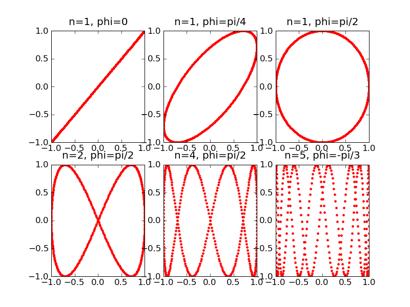
Now that we have a basic idea of plotting, let's try plotting Lissajous figures. Suppose we have two independent sinusoidal time signals $x(t)$ and $y(t)$. A Lissajous figure is a parametric plot in the form $(x,y) = (x(t), y(t))$. Such figures are useful for plotting the motion of particles under the influence of forces whose $x$ and $y$ components are independent.

Activity 3: Do the following

Write a program that will create two time series $x(t)$ and $y(t)$ over the interval $0\leq t\leq 2\pi$, with

$$x(t) = \cos(t)\quad \text{and}\quad y(t) = \cos(nt + \phi),$$

where $n$ is an integer and $\phi$ is a constant.

Try running your code for various values of $n$ and the phase constant. Use subplot to generate multiple windows, and save the output to a plot file.

Our example solution can be found here: lissajous.py. The output from this script looks like this:

Now we will look at a different type of plot: the histogram, which has its own command hist. Histograms are useful to show, for example, how often various outcomes occur in an experiment.

Activity 4: Play dice

Suppose you rolled a dice 20 times and recorded the results in an array called roll. Copy and paste the following script into a new IDLE script window and run it to make a histogram:

python code

            from pylab import *
# results of my die rolls
roll = array([2, 3, 5, 5, 4, 2, 6, 1, 2, 1, 1, 6, 2, 1, 4, 1, 3, 4, 2, 2])
# histogram
figure(1)
hist(roll)
show()

It is showing you: five times you rolled a 1, six times you rolled a 2, twice you rolled a 3, etc.

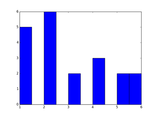
But there is a problem with this histogram: the binning, which python chooses automatically, is lousy. Inside the hist command, you can specify the number of bins immediately after the name of the array, and further change the binning using options such as range=, align=, bins=. You can then use the xticks command to control the labels on the bins.
You can also assign different weights to each bin, using the weights= option inside the hist command. For example, this allows you to "normalize" the histogram, to show you the probability of each outcome.
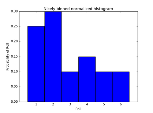
Try the following script to make a nicely-binned, normalized histogram:

python code

            from pylab import *
# results of my die rolls
roll = array([2,3,5,5,4,2,6,1,2,1,1,6,2,1,4,1,3,4,2,2])
# for normalization
N = len(roll)
weights_array = ones(N) / N
# histogram
figure(1)
hist(roll, 6, weights=weights_array, range=[0.5, 6.5], align='mid')
xticks(range(1, 7))
xlabel('Roll')
ylabel('Probability of Roll')
title('Nicely binned normalized histogram')
show()

Formatted output & tuples

In the tutorial "First Steps, Part 1" we calculated the height reached by an object projected up from the surface. We worked with these lines of code:

python code

            v=12.5
g=9.8
h=v**2/(2*g)
h

You can execute these lines of code again to remind you of what they did. The last line gives

7.9719387755102034

This number is hard to read and has far too many digits after the decimal place. To control this behaviour, we use formatted strings, which in Python requires tuples. Tuples are another type of sequence, like lists, but have a different structure and purpose. Here are some lines of code that define and explore the properties of a tuple.

python code

            # define a tuple
my_tuple = (5, 4, 3, 2, 1)
# print out some elements of my_tuple
my_tuple[0]
my_tuple[3]
# get the length of my_tuple
len(my_tuple)

A tuple is enclosed by parentheses () instead of brackets []. The elements can be accessed similarly to lists. But tuples are more hardwired than lists (they are "immutable"): you cannot change the elements of a tuple. For example, the assignment statement my_tuple[3]=-15 will give an error (try it and see).

Now that we know a bit about tuples, let's see an example of a formatted string in Python

python code

            v = 12.5
g = 9.8
h = v**2/(2*g)
h_cm = h*100
h_int = int(h)
str = "The height is {0:f} metres or {1:f} centimetres.".format(h, h_cm)
print str

Activity 5: Run this code.

This produces
The height is 7.971939 metres or 797.193878 centimetres.

In the line beginning str, the f are indicators that a floating-point number should be printed. The arguments (h, h_cm) of format indicate the values to be selected. Now, if we want to control the number of significant figures, we can use the following line to replace the str = line above:

python code

            str = "The height is {0:4.1f} metres or {1:4.1f} centimetres.".format(h, h_cm)
print str

Activity 6: Replace the string and run the new code.

This produces
The height is 8.0 metres or 797.2 centimetres.

The 4.1f strings indicate that each number should be at least four characters long and that at most one figure should be included after the decimal place. Other string-formatting codes, besides f, are s for strings, d for integers, e for floating point numbers in scientific notation exponential format. More information on string format codes can be found in our Fun with Strings page.

Activity 7: We'll repeat a prior example, produce cleaned up output, and plot the results:

Recall Activity 12 of "First Steps, Part 2", in which we found the following expressions for a particle falling under the influence of gravity and air resistance:

$$x(t) = -s_t \left[ t + \tau \left(\text{e}^{-t/\tau} -1 \right) \right],\quad v(t) = \frac{dx}{dt} = -s_t\left(1-\text{e}^{-t/\tau}\right) \quad \text{and}\quad a(t) =\frac{d^2x}{dt^2} = -\frac{s_t}\tau \text{e}^{-t/\tau}$$

We wrote the following to print out this solution:

python code

            # import numpy functions and types
from numpy import *
# define a time array
t = arange(0, 20.5, 0.5)
# terminal speed
s_t = 20.0
# time constant
tau = 5.0
# define a speed array
v = -s_t*(1-exp(-t/tau))
# define a position array
x = -s_t*(t+tau*(1-exp(-t/tau)))
# define an acceleration array
a = -s_t*exp(-t/tau)/tau
for i in range(len(t)):
    print("t, x(t), v(t), a(t)", t[i], x[i], v[i], a[i])

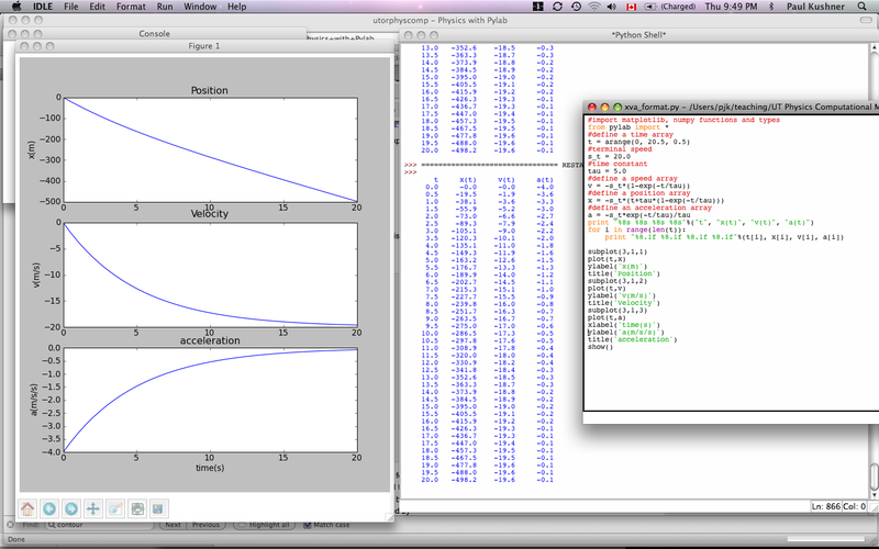
Now, modify this program to print out the program in columns with answers formatted in columns and plot the results in a manner you choose.
Our solution can be found here: xva_format.py and a screenshot of the session looks like this:

You will often need to output results to a file and read other data from an input file. We will show you a couple of tricks to get this done (ASCII output only) without dwelling on the details.

Activity 8: Writing output to a file:

Let's keep working with the falling particle example, xva.py. The following code outputs the $x(t)$, $v(t)$, and $a(t)$ to a file called xva_file.txt. Because we will use the data in xva_file.txt as input into another code in the next example, we will output the data with up to 3 digits after the decimal place (see the 8.3f format strings below).

python code

            # import pylab functions and types
from pylab import *
# This line opens the file xva_file.txt for output. The 'w' says that we are permitted to write to the file.
outfile = open('xva_file.txt', 'w')
# define a time array
t = arange(0, 20.5, 0.5)
# terminal speed
s_t = 20.0
# time constant
tau = 5.0
# define a speed array
v = -s_t*(1-exp(-t/tau))
# define a position array
x = -s_t*(t+tau*(1-exp(-t/tau)))
# define an acceleration array
a = -s_t*exp(-t/tau)/tau
str = "{0:8s} {1:8s} {2:8s} {3:8s}".format("t", "x(t)", "v(t)", "a(t)")
# print the string to the screen. A return is automatically generated.
print str
# print the string to the file, followed by a return
outfile.write(str+'\n')
for i in range(len(t)):
    str =  "{0:8.3f} {1:8.3f} {2:8.3f} {3:8.3f}".format(t[i], x[i], v[i], a[i])
    # print the string to screen
    print str
    # print the string to the file
    outfile.write(str+'\n')
 
# for loop is done. Close the file
outfile.close()

Now do the following:

Run the code above and examine the output on the screen and in the output file. A sample output file can be found here:xva_file.txt.

Activity 9: Reading input from a file:

If you carried out Activity 7, you will have a file called xva_file.txt in your run directory. How can we read the data from that file? The file starts with a header line of text followed by rows of numbers. All entries are separated by white space. For files in this format (tab, whitespace, or comma delimited), pylab provides the very handy loadtxt routine. Now do the following:

Locate the path to the file xva_file.txt. For example, it might reside under your C:\ directory on windows.
Start a new Python shell, and at the command line, type the following:
from pylab import * xva_array = loadtxt('<path to xva_file.txt>', skiprows=1)
where in the previous line, <path to xva_file.txt> is the directory path to the file you want, and skiprows=1 tells the loadtxt command to skip the first row, which contains text.
If this step worked, type the following:
xva_array
This will output a lot of numbers. If you look carefully, you will see that the numbers are consistent with the output from the xva script.
What is xva_array? It is actually a two-dimensional NumPy array of floating point numbers --- a matrix --- with 4 columns and 41 rows. To see this, type
shape(xva_array)
This will result in
(41, 4)
To understand what to do with xva_array, we will need to further explore the properties of NumPy in the next section. We will return to this example in Activity 11.

2. Working with NumPy

The NumPy module, which is a contraction of "Numerical Python", is a very important part of doing scientific computing with Python. Until we did Activity 8 in this tutorial, we were limited to one dimensional arrays, but NumPy is capable of handling multiple dimension arrays. NumPy one dimensional arrays are lists, NumPy two dimensional arrays are lists of lists, NumPy 3-d arrays are lists of lists of lists, and so on. To see how this works, do the following:

Activity 10: Creating NumPy arrays:

Reproduce the following interactive session, and include some additional commands of your own.

python code

            >>> from pylab import *  # import numpy and everything else
>>> array_1 = array([15.0, 26.0, 33.0, 34.0, 32.0, 30.0])  # create a one-d array
>>> shape(array_1)
(6,)
>>> array_2 = zeros(3)
>>> array_2
array([ 0.,  0.,  0.])
>>> array_3 = zeros((3,4))
>>> array_3
array([[ 0.,  0.,  0.,  0.],
       [ 0.,  0.,  0.,  0.],
       [ 0.,  0.,  0.,  0.]])
>>> array_4 = ones((3,4,2))
>>> array_4
array([[[ 1.,  1.],
        [ 1.,  1.],
        [ 1.,  1.],
        [ 1.,  1.]],
 
       [[ 1.,  1.],
        [ 1.,  1.],
        [ 1.,  1.],
        [ 1.,  1.]],
 
       [[ 1.,  1.],
        [ 1.,  1.],
        [ 1.,  1.],
        [ 1.,  1.]]])
>>> shape(array_3)
(3, 4)
>>> shape(array_4)
(3, 4, 2)

Notice the following:

The numpy module allows you to initialize arrays full of zeros or ones.
The shape is determined by a sequence like (3, 4, 2) --- you can also use [3, 4, 2] --- and this shape can be accessed using the shape function.
The numpy multidimensional arrays are implemented as nested lists.

Activity 11: Working with numpy arrays:

The numpy module has very useful array indexing features and ways to manipulate the shapes of arrays. Try to reproduce the following session, including the error we made!

python code

            >>> array_1  # the original array
array([ 15.,  26.,  33.,  34.,  32.,  30.])
>>> array_1.reshape((2, 3))  # a reshaped version of the array into a 2 by 3 matrix
array([[15.,  26., 33.],
       [34.,  32., 30.]])
>>> array_4 = array_1.reshape((2, 3))
>>> array_4
array([[15., 26., 33.],
       [34., 32., 30.]])
>>> shape(array_4) #what is the new shape of array_4?
(2, 3)
>>> array_4[0, :] #the first row of array_4
array([15., 26., 33.])
>>> array_4[:, 1] #the second column of array_4
array([26., 32.])
>>> array_4[2, 1] #the element at the third row and the second column of array_4. Oops!
Traceback (most recent call last):
  File "<pyshell#84>", line 1, in <module>
    array_4[2, 1]
IndexError: index (2) out of range (0<=index<2) in dimension 0
>>> array_4[1, 2]  # the element at the third column and the second row of array_4
30.0

Note that for a two-dimensional array a, a[:, j] is row j+1 of the array, and a[k, :] is column k+1 of the array.

Given what we know about NumPy arrays, we can now better handle pylab's loadtxt command. Here is the procedure to read in a comma or blank-separated ASCII file of values.

Look at the file and identify its overall structure.
Run the loadtxt command, skipping any header rows that contain text.
Check the shape of the resulting array, which will tell you the number of rows and columns.
Extract rows and columns as appropriate.

Here's this procedure in action

Activity 12 Loading a blank-separated ascii file, part 2.

Do the following:

Write a script to read in and plot the data from xva_file.txt.
Use Activity 8 to guide you. The xva_array, whose shape is 41 by 4, has columns that correspond to t, x(t), v(t), a(t).
Now plot the data, including the following lines of code in your script:
t = xva_array[:, 0] x = xva_array[:, 1] v = xva_array[:, 2] a = xva_array[:, 3]
See if you can reproduce the plots of the position, velocity and acceleration from before.
Our solution script can be found here: xva_from_input_file.py. Note that the path to the xva_array.txt file will be different for you. If the file you want to load is in the same folder as your script, then identifying the full path is unnecessary (i.e. just 'xva_array.txt' will work).

Here are some questions to practice graphing with Pylab:
graphing.questions.pdf
graphing.solutions.pdf

OTHER MATERIAL
*
*

Given the velocity, the position and acceleration are obtained by

These equations represent the exact solution to the problem. But we also want to calculate these quantities numerically. To do this, we need to find numerical approximations to derivatives and integrals. We will use the simplest formulas to proceed.

First, to find an approximate solution for the position, we recall from calculus that the velocity v(t) is defined by

This means that

with the approximation becoming more accurate as

gets smaller. So to find the position as a function of time numerically we start at the initial position x(0)=0 and update to the next time according to the approximate formula

and update to subsequent times according to

This is equivalent to finding the integral as a (right) Riemann sum.

Second, to find an approximate solution for the acceleration, we recall that the acceleration a(t) is defined by

This means that

So to find the acceleration as a function of time numerically we use the approximate formula