Tutorial, Part 5: NumPy, SciPy, and Matplotlib

Contact: compwiki@physics.utoronto.ca

1. Numpy and numpy arrays

We will be making a great deal of use of the array structures found in the numpy package. These arrays are used in many python packages used in computational science, data analysis, and graphical analysis (in packages like scipy and matplotlib).

Numpy arrays are a type of highly structured list that you can use for doing common numerical and matrix calculations.

While there are exceptions, numpy arrays are a special kind of list with a constrained size and with all entries having the same type.
Numpy arrays make it easy to set up vectors, matrices, and higher order tensor objects for further manipulation.
Importantly, Python has optimized its handling of numpy arrays to carry out calculations very quickly and efficiently.
All told, hey are very handy for computational physics.

To created numpy arrays, we first need to import the numpy module as follows: either

python code

            import numpy as np

or, more conveniently (though not recommended)

python code

            from numpy import *

The first statement imports numpy as renames it to np. You can rename any module in this way and this is a common renaming for numpy. Then individual methods and objects within numpy can be referred to as follows: np.sin(), np.pi, etc..
The second statement imports everything related to numpy and allows you to simply use sin(), pi, etc.

The first statement is preferable:

It keeps all of numpy within its own namespace, so you are always aware that you're using a numpy function instead of your own function, and avoids conflicts with other implementations of the same functions in other packages (scipy, sympy, math...)
It is the standard method in the scientific Python community. Any documentation you find on the internet will likely use import numpy as np.

Activity 1: Do the following

Enter the following commands one at a time and examine the output:

python code

            import numpy as np
a = np.array([0, 10, 20, 30, 40])
a
a[:]
a[1:3]
a[1] = 15
a
b = np.arange(-5, 5, 0.5)
b
b**2
1/b
1/b[10]

The output from the session is

python code

            In [4]: import numpy as np
In [5]: a = np.array([0, 10, 20, 30, 40])
In [6]: a
Out[6]: np.array([ 0, 10, 20, 30, 40])
In [7]: a[:]
Out[7]: np.array([ 0, 10, 20, 30, 40])
In [8]: a[1:3]
Out[8]: np.array([10, 20])
In [9]: a[1] = 15
In [10]: a
Out[10]: np.array([ 0, 15, 20, 30, 40])
In [11]: b = np.arange(-5, 5, 0.5)
In [12]: b
Out[12]: np.array([-5. , -4.5, -4. , ...,  3.5,  4. ,  4.5])
In [13]: b**2
Out[13]: np.array([ 25.  ,  20.25,  16.  , ...,  12.25,  16.  ,  20.25])
In [14]: 1/b
__main__:1: RuntimeWarning: divide by zero encountered in true_divide
Out[14]: 
array([-0.2       , -0.22222222, -0.25      , ...,  0.28571429,
        0.25      ,  0.22222222])
...
In [20]: b[10]
Out[20]: 0.0
In [21]: 1/b[10]
__main__:1: RuntimeWarning: divide by zero encountered in double_scalars
Out[21]: inf

Now do the following:

Look carefully at the output of the arange command, and make sure you understand it. To get more explanation on arange, type help(arange).
Notice that operations on numpy arrays act on each element in the array. So b**2 has the effect of raising to the power of two each element in the array.
Notice that the divide by zero in the 1/b command results in an "Inf" output, located at element [10].
You can practice further with numpy arrays. For example, create another array c=0.5*b, and then type b + c. Notice that for numpy arrays, b + c is not a concatenation of two lists, as in our previous discussion of lists, but the sum of the elements of b and c. (This example shows how Python interprets operators like + in the context of the operands, i.e. the objects that are involved in the operation. This reflects the object-oriented character of Python.)

Activity 2: To further practice using numpy arrays, do the following example:

Suppose an object under the influence of gravity and resistive drag falls with a downward velocity $ v(t) = -s_t\left(1 - \exp(-\frac{t}{\tau})\right) $ where $ s_t $ is the terminal speed and $\tau=5$ is a time constant. Write a program to write the acceleration and position of the object every half second for 20 seconds. Assume the initial position $x(0)=0$. (We will use this example to illustrate a few other ideas after we're done.)

We first find analytic expressions for the position and acceleration. Given the velocity, the position and acceleration are obtained from integration and differentiation by:

$$x(t) = \int_0^t v(t')dt'+x(0)=-s_t\left[t+\tau(e^{-t/\tau} -1\right]$$

and $ a(t) = \frac{dv}{dt} = -\frac{s_t}{\tau}e^{-t}{\tau} $

Our script imports numpy and defines a time array t with the following line:

python code

            t = np.arange(0,20.5,0.5)

Another standard trick is to create a for loop that will run over an index that extends from the beginning to the end of an array. For example, to create a code that prints the elements of t[:], we write

python code

            for j in range(len(t)): print(t[j])

To make sure you understand the previous line code example: len(t) is the length of the array t, which is 41. range(len(t)) is an array of integers [0, 1, 2 ..., 39, 40].The for header creates a variable j that iterates over range(len(t)). In the body of the loop, t[j] is the j^th value of t.

Now go ahead and produce a solution on your own, then check your answer against this script, which you can download and run.

2. Matplotlib

Plotting figures is an essential part of using Python for physics research and learning. The main plotting package is python is called matplotlib. The odd name comes from the the fact that the plotting interface is modelled after the (non-free) computation program matlab. Matplotlib has evolved since it was first created and has influenced plotting code for many newer plotting packages, like bokeh, plotly, ggplot (the Python version).

Matplotlib can be imported in a few ways.

python code

            import matplotlib
import pylab
import matplotlib.pyplot

The first import (matplotlib) imports the entire package, the second imports only the core plotting interface (pyplot), the third imports (pylab) a special package that includes plotting (pyplot) and numerical methods (numpy). Note that the use of PyLab is typically discouraged. One common way of importing matplotlib and numpy is to use

python code

            import numpy as np
import matplotlib.pyplot as plt

This will making the plotting available as the prefix plt and numpy available as np.

The simplest plot command is

python code

            import matplotlib.pyplot as plt
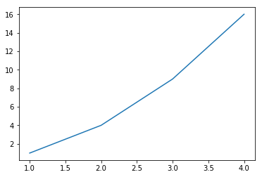
plt.plot([1, 2, 3, 4], [1, 4, 9, 16])
plt.show()

This code will simply plot the elements of the list [1, 2, 3, 4] against the elements other list [1, 4, 9, 16]. Depending on your Spyder or Jupyter configuration, the final command in your plotting might need to be show(), which activates the plotting window.

Activity 1: Copy and save the excerpt above to a new script file, and run it in Spyder using F5. The result should be a window like this

To learn more about the very powerful plot command, in the Python shell type

python code

            from pylab import *
help(plot)

but, as with many matplotlib commands, the documentation is extensive and is helped by seeing examples of the usage. You can visit matplotlib.org to get the same documentation and see examples from the gallery.

The following activity will help you explore several useful capabilities of matplotlib.

Activity 2: Do the following:

Copy and paste the following script into a new Spyder script window and run it.
Inspect the plotted figure, then quickly read over the code, trying to get an overall understanding of the different commands.
For guidance on the commands, checking the matplotlib website, or type from pylab import * in the Python shell and use help() on the commands. This is a quick way to learn about the capabilities of PyLab.

python code

            # import numpy functions and types
from pylab import *
x = arange(1, 10, 0.5)
xsquare = x**2
xcube = x**3
xsquareroot = x**0.5
# open figure 1
figure(1)
# basic plot
plot(x, xsquare)
# add a label to the x axis
xlabel('abscissa')
# add a label to the y axis
ylabel('ordinate')
# add a title
title('A practice plot.')
# save the figure to the current diretory as a png file
savefig('plot_1.png')
# open a second figure
figure(2)
# do two plots:
# one with red circles with no line joining them
# and another with green plus signs joined by a dashed curve
plot(x, xsquare, 'ro', x, xcube,'g+--')
# x and y labels, title
xlabel('abscissa')
ylabel('ordinate')
title('More practice.')
# add a legend
legend(('squared', 'cubed'))
# save the figure
savefig('plot_2.png')
figure(3)
# use the subplot function to generate multiple panels within the same plotting window
subplot(3,1,1)
# plot black stars with dotted lines
plot(x, xsquareroot,'k*:')
title('square roots')
subplot(3,1,2)
# plot red right-pointing triangles with dashed lines
plot(x, xsquare,'r>-')
title('squares')
subplot(3,1,3)
# plot magenta hexagons with a solid line
plot(x, xcube,'mh-')
title('cubes')
savefig('plot_3.png')
# show() should be the last line
show()

3. Scipy

Scipy, or Scientific Python, is the last package in this part of the tutorial. scipy is a collection of functions to perform basic scientific programming and data analysis. It is also the ecosystem for many other scientific packages and provides a consistent interface to the functions and avoids duplication. For example, scipy contains Fourier transforms (scipy.fftpack), and numerical integration (scipy.integrate). It also provides the core functions for machine learning (scikit-learn) and image processing (scikit-image).

For example, to integrate a list of numbers using scipy you might use a function called trapz (for trapezoid, the type of integration being used) from the integrate package.

python code

            import scipy.integrate as integrate
result = integrate.trapz([0, 1, 2, 3, 4, 5])
print(result)
# 12.5

or if you wanted to integrate $sin(x)$ from 0 to $\pi$ you could use the quad (short for quadrature) function

python code

            import numpy as np
import scipy.integrate as integrate
result = integrate.quad(np.sin, 0, np.pi)
print(result)
# (2.0, 2.220446049250313e-14)

Here, quad takes a function name (e.g. np.sin) and the limits of the integral, but no data points. Scipy then tries to integrate the function and returns two values. The first value is the answer, the second value is an estimate of the error in the answer.

Optimization

Another common use for scipy is optimization using the scipy.optimize package. This is the package used to fit data to scientific models, or fitting values to polynomials. One way of fitting data is to use the curve_fit function, which takes at least three arguments

The function that you want to fit.
A set of independent data.
A set of dependent data.

The data you give curve_fit could be collected from an experiment, for example. You can also give curve_fit some additional help if your function is particularly complex. For example

You can provide initial guesses for your function in a keyword p0.
You can give relative or absolute errors on your dependent data using the keyword sigma (and absolute_sigma).

Activity 3: Copy and the code below into Spyder. What does it do? Run it and check the output.

python code

            import scipy.optimize as optimize
import numpy as np

def quadratic(x, a, b, c):
    return a*x**2 + b*x + c

xdata = [0, 1, 2, 3, 4, 5]
ydata = [0, 1.1, 3.8, 9.1, 15.8, 25.4]

popt, pcov = optimize.curve_fit(quadratic, xdata, ydata)

print(popt[0], "+-", pcov[0, 0]**0.5)
print(popt[1], "+-", pcov[1, 1]**0.5)
print(popt[2], "+-", pcov[2, 2]**0.5)
# 1.0446428571429547 +- 0.03670934671273757
# -0.18321428571686704 +- 0.19121776230283158
# 0.08214285714085645 +- 0.20328717992060147

The code does a few new things.

It defines a function quadratic that calculates a quadratic function as $ y=ax^2 + bx + c $.
We 'generated' some data in xdata and ydata. ydata has some small 'experimental' errors.
We used curve_fit to find values for the parameters a, b, and c in the quadratic function.

Curve fit always returns 2 things to you. The first (we've called popt) is the optimized values for the parameters. In this case the best estimate of values for a, b, and c. The second (we've called pcov) is the covariance matrix of errors in the optimized values. This matrix is square with the number of rows matching the number of parameters. The most important elements of the matrix are the diagonal elements that give you the variance in the estimated parameters, which you can use as an estimate on the size of error in your calculation.

The last three lines print the values of the parameters with their standard deviations (square root of the variance). The fitted equation is roughly $ y = (1.04 \pm 0.04)x^2 - (0.2\pm 0.2)x + (0.08\pm0.2) $. The data used in this example is simply $ y=1x^2 + 0x + 0 $ with a small error.

Activity 3: measuring gravity

A more complex example, might be to use a ball dropping in a vacuum to find the acceleration due to gravity. For this experiment the equation would be

$$h = \frac{1}{2}gt^2$$

If you know the ball was dropped 6 times from (exactly) 1 metre, and the times were 0.814, 0.741, 0.694, 0.618, 0.725, 0.753 seconds, with an error on each measurement of 0.1 seconds. How would you write the code you calculate gravity? What number would you write for the value (Python will happily print out sixteen digits even when you don't have that accuracy in your data). Our solution is below

python code

            import scipy.optimize as optimize
import numpy as np

def gravity(x, g):
    return np.sqrt(2*x/g)

xdata = [1, 1, 1, 1, 1, 1]  # height in metres
ydata = [0.814, 0.741, 0.694, 0.618, 0.725, 0.753]  # time in seconds
sigma = [0.1, 0.1, 0.1, 0.1, 0.1, 0.1]  # errors in seconds
# we use sigma and absolute sigma so that we get the correct error values
popt, pcov = optimize.curve_fit(gravity, xdata, ydata, sigma=sigma, absolute_sigma=True) 

print(popt[0], "+-", pcov[0,0]**0.5)

and the value of gravity is $ g = 3.81 \pm 0.43 m\,s^{-2}$. If you don't use sigma and absolute_sigma in your code, you might get $ g = 3.81 \pm 0.28 m\,s^{-2}$, which has a smaller error but is not correct.

4. Recap

This concludes the Part 5 of the tutorial. In summary:

We have learned about numpy arrays like np.array([1,2,3,4,5]) and what kind of operations can be done on them.
We have learned how to explore possible actions on an object with dir(my_object) and help(my_object.method)
We have learned about for plotting data with pylab and matplotlib.
We have begun to explore the scientific package scipy and used it to fit a model of the world to our experimental data.

We hope that this tutorial has helped start you on the path to doing physics with computers. Please speak to your instructor if you have any suggestions for how to improve this tutorial.