You will probably encounter many situations in which analytical integration of a function or a differential equation is difficult or impossible. In this section we show how Scientific Python can help through its high level mathematical algorithms. You will learn how to develop you own numerical integration method and how to get a specified accuracy. The package scipy.integrate can do integration in quadrature and can solve differential equations

1. The Basic Trapezium Rule

Scipy uses three methods to integrate a one-dimensional function: trapezoidal (integrate.trapz), Simpson (integrate.simps) and Romberg (integrate.romb). The trapezium (trapezoidal) method is the most straightforward of the three. The simple trapezium formula calculates the integral of a function f(x) as the area under the curve representing f(x) by approximating it with the sum of trapeziums:

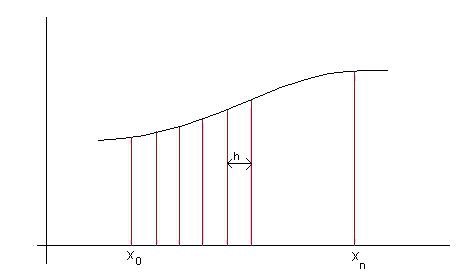
The area of each trapezium is calculated as width times the average height.
Example: Evaluate the integral:

using the basic trapezium rule.
We shall write a small program to evaluate the integral. Of course we have to estimate the number of trapeziums to use; the accuracy of our method depends on this number.

            import math
#the function to be integrated:
def f(x):
    return x ** 4 * (1 - x) ** 4 / (1 + x ** 2)
 
#define a function to do integration of f(x) btw. 0 and 1:
def trap(f, n):
    h = 1 / float(n)
    intgr = 0.5 * h * (f(0) + f(1))
    for i in range(1, int(n)):
        intgr = intgr + h * f(i * h)
    return intgr
 
print(trap(f, 100))
        

Our basic integration program has the inconvenience of depending on the number of trapeziums that we have to change manually. As a basic rule, if we double the number of trapeziums and get the same answer within 1 in 1000000, the answer is probably correct.

Activity 1:

Run the program. How many trapeziums are needed to get a relative error of less than 1 part in 1,000,000?
We can do this as follows:

            from math import *
n = 1
while abs(trap(f, n) - trap(f, n * 2)) > 1e-6:
    n += 1
print(n)
        

After running this code you should end up with a printed out value of 6.

Activity 2: Calculate

\[ \int_{-\infty}^\infty e^{-x^2} dx\]

You have to modify the previous program because of the infinite range of integration. Check the integrand to see where it becomes negligible. The modified code should look something like this.

            import math
#the function to be integrated:
def f(x):
    return math.exp(-x**2)
 
#define a function to do integration of f(x) btw. a and b:
def trap(f, n, a, b):
    h = (b - a) / float(n)
    intgr = 0.5 * h * (f(a) + f(b))
    for i in range(1, int(n)):
        intgr = intgr + h * f(a + i * h)
    return intgr
 
a = -10
b = 10
n = 100
 
while(abs(trap(f, n, a, b) - trap(f, n * 4, a * 2, b * 2)) > 1e-6):
    n *= 4
    a *= 2
    b *= 2
 
print(trap(f, n, a, b))
        

And the printed result when the program is run should be something close to 1.77245385091.

2. Integrating a function with scipy.integrate

Let's look at:

Our simple integration program will divide the interval 0 to 2 in equally spaced slices and spend the same time calculating the integrand in each of these slices. If we have a closer look at the integrand and plot it, we would notice that at low x-values the function hardly varies, so our program will waste time in that region. In contrast, the integrate.quad() routine from Scipy is arbitrary callable (adaptive), in the sense that it can adjust the function evaluations to concentrate on the more important regions (quad is short for quadrature, an older name for integration). Let’s see how Scipy could simplify our work:

            import scipy
from scipy.integrate import quad
from math import *
 
def f(x):
    return x ** 4 * log(x + sqrt(x ** 2 + 1))
 
print(quad(f, 0, 2))
        

The output will be (8.153364119811167, 9.0520525739669813e-014). As you notice, we get both the integral value and the error estimate in only three lines of code, without bothering about the number of trapeziums or the accuracy. The integrate.quad() routine takes the function and the integration limits as input arguments.An overview of scipy.integrate modules can be accessed by typing in the shell window:

            >>> from scipy import integrate
>>> help(integrate)
        

Activity 3:

The period of a pendulum of length l oscillating at a large angle α is given by

where

is the period of the same pendulum at small amplitudes. In Exercises 2 and 3 you will analyze both experimental data and the Pylab plot of the large-angle pendulum. Any numerical evaluation of the integral as is would fail (explain why). If we change the variable by writing:

we can get:

which is a well-behaved integral. Write a program to use the above integral to calculate the ratio T/T0 for integral amplitudes 0° ≤ α ≤ 90°. Output these values as a table showing the amplitude in degrees and radians as well as T/T0. Explain the result when α = 0. Think about this for a moment before you read the solution below.

            from pylab import *
from math import *
import scipy
from scipy.integrate import quad
 
#the function to be integrated:
def f(x, a):
    return(2/pi)/sqrt(1-sin(a/2)**2*sin(x)**2)
 
print("%15s%15s%15s" % ("A (degrees)", "A (radians)", "T/T0"))
for i in range(0, 91):
    angle = pi * i / 180
    print("%15d%15.10f%15.10f" % (i, angle, quad(f,0,pi/2,args=(angle))[0]))
        

Some sample output can be found here. NumIntA3output.txt

Activity 4:

On the same graph, compare the plot of the sin function with the plot of the integral of the cos function in the range [-π, π].
This can be done as follows:

            from pylab import *
from math import *
import scipy
from scipy.integrate import quad
 
#the function to be integrated:
def f(x):
    return cos(x)
 
x = arange(-pi, pi + 0.1, 0.1)
y_sin = []
y_cos_integrated = []
 
for element in x:
    y_sin.append(sin(element))
    y_cos_integrated.append(quad(f, -pi, element)[0] - sin(pi))
 
plot(x, y_sin)
plot(x, y_cos_integrated)
show()
        

3. Integrating ordinary differential equations with odeint

Many physical phenomena are modeled by differential equations: oscillations of simple systems (spring-mass, pendulum, etc.), fluid mechanics (Navier-Stokes, Laplace's, etc.), quantum mechanics (Schrödinger’s) and many others. Here we’ll show you how to numerically solve these equations. The example we shall use in this tutorial is the dynamics of a spring-mass system in the presence of a drag force.

Writing Newton’s second law for the system, we have to combine the elastic force

with the drag force whose model for a slowly moving object is

We obtain the formula

or

where L is the length of the unstretched/uncompressed spring.

To find an approximate solution to the equation of motion above, we’ll have to use a finite difference approximation for the derivative, which will generate an algorithm for solving the equation. Most such algorithms are based on first order differential equations, so it will probably not be a bad idea to start by putting our second-order equation in the form of a system of two first-order differential equations:

To write the numerical integration program, we shall use odeint, which is part of scipy.integrate. A function call to odeint looks something like this:

            scipy.integrate.odeint(func, y0, t, args=())
        

As you may see in the simplified syntax above, it takes a number of input arguments: function func defining the system of first order equations, initial values of variables y0 (put in an array), time t (an array of time values), and arguments args() which can be our parameters (mass, elastic constant, drag coefficient and initial length of the spring). The unknowns in a system of differential equations are functions; odeint will return to us the values of these functions at the values t provided, as an array.

Here is how we construct such a program:

            from scipy import *
from scipy.integrate import odeint
from pylab import *
 
"""
A spring-mass system with damping
"""
 
def damped_osc(u,t): #defines the system of diff. eq.
    x, v = u
    return(v,-k*(x-L)/m-b*v) #the vector (dx/dt, dv/dt)
 
t = arange(0,20.1,0.1)
u0 = array([1,0])   #initial values of x, v
 
#assume certain values of parameters b, k, L, m; these would be given in the problem
b=0.4
k=8.0
L=0.5
m=1.0
 
u=odeint(damped_osc,u0,t) #solve ODE
#plot x, v, phase, using matplotlib
 
figure(1)
plot(t,u[:,0],t,u[:,1]) #u[:,0] is x; u[:,1] is v
xlabel('Time')
title('Damped Oscillator')
 
figure(2)
plot(u[:,0],u[:,1])
title('Phase-space')
xlabel('Position')
ylabel('Velocity')
show()
        

The phase-space plot shows the characteristic non-conservative spiral shape, while the displacement and velocity graphs show the expected damping. Practice numerical integration and solving differential equations with the following exercises:
numerical_integration.questions.pdf
numerical_integration.solutions.pdf